const matrix = [_]u8{
    201, 10, 25, 185, 65, 70,
    65, 120, 110, 65, 120, 117,
    98, 95, 12, 213, 26, 88,
    143, 112, 65, 97, 99, 205,
    234, 105, 56, 43, 44, 216,
    45, 59, 243, 211, 209, 54,
};15 Project 4 - Developing an image filter
In this chapter we are going to build a new project. The objective of this project is to write a program that applies a filter over an image. More specifically, a “grayscale filter”, which transforms any color image into a grayscale image.
We are going to use the image displayed in Figure 15.1 in this project. In other words, we want to transform this colored image into a grayscale image, by using our “image filter program” written in Zig.

We don’t need to write a lot of code to build such “image filter program”. However, we first need to understand how digital images work. That is why we begin this chapter by explaining the theory behind digital images and how colors are represented in modern computers. We also give a brief explanation about the PNG (Portable Network Graphics) file format, which is the format used in the example images.
At the end of this chapter, we should have a full example of a program that takes the PNG image displayed in Figure 15.1 as input, and writes a new image to the current working directory that is the grayscale version of this input image. This grayscale version of Figure 15.1 is exposed in Figure 15.2. You can find the full source code of this small project at the ZigExamples/image_filter folder at the official repository of this book1.

15.1 How we see things?
In this section, I want to briefly describe to you how we (humans) actually see things with our own eyes. I mean, how our eyes work? If you do have a very basic understanding of how our eyes work, you will understand more easily how digital images are made. Because the techniques behind digital images were developed by taking a lot of inspiration from how our human eyes work.
You can interpret a human eye as a light sensor, or, a light receptor. The eye receives some amount of light as input, and it interprets the colors that are present in this “amount of light”. If no amount of light hits the eye, then, the eye cannot extract color from it, and as result, we end up seeing nothing, or, more precisely, we see complete blackness.
Therefore, everything depends on light. What we actually see are the colors (blue, red, orange, green, purple, yellow, etc.) that are being reflected from the light that is hitting our eyes. Light is the source of all colors! This is what Isaac Newton discovered on his famous prism experiment2 in the 1660s.
Inside our eyes, we have a specific type of cell called the “cone cell”. Our eye have three different types, or, three different versions of these “cone cells”. Each type of cone cell is very sensitive to a specific spectrum of the light. More specifically, to the spectrums that define the colors red, green and blue. So, in summary, our eyes have specific types of cells that are highly sensitive to these three colors (red, green and blue).
These are the cells responsible for perceiving the color present in the light that hits our eyes. As a result, our eyes perceives color as a mixture of these three colors (red, green and blue). By having an amount of each one of these three colors, and mixing them together, we can get any other visible color that we want. So every color that we see is perceived as a specific mixture of blues, greens and reds, like 30% of red, plus 20% of green, plus 50% of blue.
When these cone cells perceive (or, detect) the colors that are found in the light that is hitting our eyes, these cells produce electrical signals, which are sent to the brain. Our brain interprets these electrical signals, and use them to form the image that we are seeing inside our head.
Based on what we have discussed here, the bullet points exposed below describes the sequence of events that composes this very simplified version of how our human eyes work:
- Light hits our eyes.
- The cone cells perceive the colors that are present in this light.
- Cone cells produce electrical signals that describes the colors that were perceived in the light.
- The electrical signals are sent to the brain.
- Brain interprets these signals, and form the image based on the colors identified by these electrical signals.
15.2 How digital images work?
A digital image is a “digital representation” of an image that we see with our eyes. In other words, a digital image is a “digital representation” of the colors that we see and perceive through the light. In the digital world, we have two types of images, which are: vector images and raster images. Vector images are not described here. So just remember that the content discussed here is related solely to raster images, and not vector images.
A raster image is a type of digital image that is represented as a 2D (two dimensional) matrix of pixels. In other words, every raster image is basically a rectangle of pixels, and each pixel have a particular color. So, a raster image is just a rectangle of pixels, and each of these pixels are displayed in the screen of your computer (or the screen of any other device, e.g. laptop, tablet, smartphone, etc.) as a color.
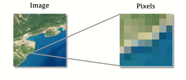
Figure 15.3 demonstrates this idea. If you take any raster image, and you zoom into it very hard, you will see the actual pixels of the image. JPEG, TIFF and PNG are file formats that are commonly used to store raster images.
The more pixels the image has, the more information and detail we can include in the image. The more accurate, sharp and pretty the image will look. This is why photographic cameras usually produce big raster images, with several megapixels of resolution, to include as much detail as possible into the final image. As an example, a digital image with dimensions of 1920 pixels wide and 1080 pixels high, would be a image that contains \(1920 \times 1080 = 2073600\) pixels in total. You could also say that the “total area” of the image is of 2073600 pixels, although the concept of “area” is not really used here in computer graphics.
Most digital images we see in our modern world uses the RGB color model. RGB stands for (red, green and blue). So the color of each pixel in these raster images are usually represented as a mixture of red, green and blue, just like in our eyes. That is, the color of each pixel is identified by a set of three different integer values. Each integer value identifies the “amount” of each color (red, green and blue). For example, the set (199, 78, 70) identifies a color that is more close to red. We have 199 of red, 78 of green, and 70 of blue. In contrast, the set (129, 77, 250) describes a color that is more close to purple. Et cetera.
15.2.1 Images are displayed from top to bottom
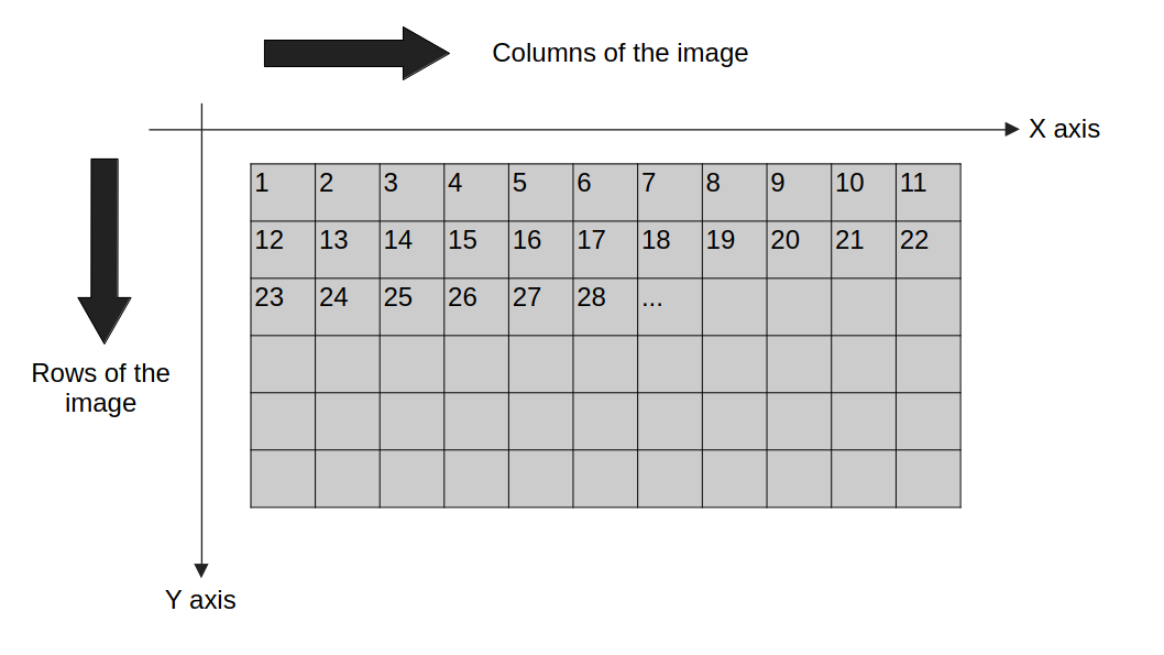
This is not a rule written in stone, but the big majority of digital images are displayed from top to bottom and left to right. Most computers screens also follow this pattern. So, the first pixels in the image are the ones that are at the top and left corner of the image. You can find a visual representation of this logic in Figure 15.4.
Also notice in Figure 15.4 that, because a raster image is essentially a 2D matrix of pixels, the image is organized into rows and columns of pixels. The columns are defined by the horizontal x axis, while the rows are defined by the vertical y axis.
Each pixel (i.e., the gray rectangles) exposed in Figure 15.4 contains a number inside of it. These numbers are the indexes of the pixels. You can notice that the first pixels are in the top and left corner, and also, that the indexes of these pixels “grow to the sides”, or, in other words, they grow in the direction of the horizontal x axis. Most raster images are organized as rows of pixels. Thus, when these digital images are displayed, the screen display the first row of pixels, then, the second row, then, the third row, etc.
15.2.2 Representing the matrix of pixels in code
Ok, we know already that raster images are represented as 2D matrices of pixels. But we do not have a notion of a 2D matrix in Zig. Actually, most low-level languages in general (Zig, C, Rust, etc.) do not have such notion. So how can we represent such matrix of pixels in Zig, or any other low-level language? The strategy that most programmers choose in this situation is to just use a normal 1D array to store the values of this 2D matrix. In other words, you just create an normal 1D array, and store all values from both dimensions into this 1D array.
As an example, suppose we have a very small image of dimensions 4x3. Since a raster image is represented as a 2D matrix of pixels, and each pixel is represented by 3 “unsigned 8-bit” integer values, we have 12 pixels in total in this image, which are represented by \(3 \times 12 = 36\) integer values. Therefore, we need to create an array of 36 u8 values to store this small image.
The reason why unsigned 8-bit integer (u8) values are used to represent the amounts of each color, instead of any other integer type, is because they take the minimum amount of space as possible, or, the minimum amount of bits as possible. Which helps to reduces the binary size of the image, i.e., the 2D matrix. Also, they convey a good amount of precision and detail about the colors, even though they can represent a relatively small range (from 0 to 255) of “color amounts”.
Coming back to our initial example of a 4x3 image, the matrix object exposed below could be an example of an 1D array that stores the data that represents this 4x3 image.
The first three integer values in this array are the color amounts of the first pixel in the image. The next three integers are the colors amounts for the second pixel. And the sequence goes on in this pattern. Having that in mind, the size of the array that stores a raster image is usually a multiple of 3. In this case, the array have a size of 36.
I mean, the size of the array is usually a multiple of 3, because in specific circumstances, it can also be a multiple of 4. This happens when a transparency amount is also included into the raster image. In other words, there are some types of raster images that uses a different color model, which is the RGBA (red, green, blue and alpha) color model. The “alpha” corresponds to an amount of transparency in the pixel. So every pixel in a RGBA image is represented by a red, green, blue and alpha values.
Most raster images uses the standard RGB model, so, for the most part, you will see arrays sizes that are multiples of 3. But some images, especially the ones that are stored in PNG files, might be using the RGBA model, and, therefore, are represented by an array whose size is a multiple of 4.
In our case here, the example image of our project (Figure 15.1) is a raster image stored in a PNG file, and this specific image is using the RGBA color model. Therefore, each pixel in the image is represented by 4 different integer values, and, as consequence, to store this image in our Zig code, we need to create an array whose size is a multiple of 4.
15.3 The PNG library that we are going to use
Let’s begin our project by focusing on writing the necessary Zig code to read the data from the PNG file. In other words, we want to read the PNG file exposed in Figure 15.1, and parse its data to extract the 2D matrix of pixels that represents the image.
As we have discussed in Section 15.2.2, the image that we are using as example here is a PNG file that uses the RGBA color model, and, therefore, each pixel of the image is represented by 4 integer values. You can download this image by visiting the ZigExamples/image_filter folder at the official repository of this book3. You can also find in this folder the complete source code of this small project that we are developing here.
There are some C libraries available that we can use to read and parse PNG files. The most famous and used of all is libpng, which is the “official library” for reading and writing PNG files. Although this library is available on most operating system, it’s well known for being complex and hard to use.
That is why, I’m going to use a more modern alternative here in this project, which is the libspng library. I choose to use this C library here, because it’s much, much simpler to use than libpng, and it also offers very good performance for all operations. You can checkout the official website of the library4 to know more about it. You will also find there some documentation that might help you to understand and follow the code examples exposed here.
First of all, remember to build and install this libspng into your system. Because if you don’t do this step, the zig compiler will not be able to find the files and resources of this library in your computer, and link them with the Zig source code that we are writing together here. There is good information about how to build and install the library at the build section of the library documentation5.
15.4 Reading the PNG file
In order to extract the pixel data from the PNG file, we need to read and decode the file. A PNG file is just a binary file written in the “PNG format”. Luckily, the libspng library offers a function called spng_decode_image() that does all this heavy work for us.
Now, since libspng is a C library, most of the file and I/O operations in this library are made by using a FILE C pointer. Because of that, is probably a better idea to use the fopen() C function to open our PNG file, instead of using the openFile() method that I introduced in Chapter 13. That is why I’m importing the stdio.h C header in this project, and using the fopen() C function to open the file.
If you look at the snippet below, you can see that we are:
- opening the PNG file with
fopen(). - creating the
libspngcontext withspng_ctx_new(). - using
spng_set_png_file()to specify theFILEobject that reads the PNG file that we are going to use.
Every operation in libspng is made through a “context object”. In our snippet below, this object is ctx. Also, to perform an operation over a PNG file, we need to specify which exact PNG file we are referring to. This is the job of spng_set_png_file(). We are using this function to specify the file descriptor object that reads the PNG file that we want to use.
const c = @cImport({
    @cDefine("_NO_CRT_STDIO_INLINE", "1");
    @cInclude("stdio.h");
    @cInclude("spng.h");
});

const path = "pedro_pascal.png";
const file_descriptor = c.fopen(path, "rb");
if (file_descriptor == null) {
    @panic("Could not open file!");
}
const ctx = c.spng_ctx_new(0) orelse unreachable;
_ = c.spng_set_png_file(
    ctx, @ptrCast(file_descriptor)
);
Before we continue, is important to emphasize the following: since we have opened the file with fopen(), we have to remember to close the file at the end of the program, with fclose(). In other words, after we have done everything that we wanted to do with the PNG file pedro_pascal.png, we need to close this file, by applying fclose() over the file descriptor object. We could use also the defer keyword to help us in this task, if we want to. This code snippet below demonstrates this step:
if (c.fclose(file_descriptor) != 0) {
    return error.CouldNotCloseFileDescriptor;
}
15.4.1 Reading the image header section
Now, the context object ctx is aware of our PNG file pedro_pascal.png, because it has access to a file descriptor object to this file. The first thing that we are going to do is to read the “image header section” of the PNG file. This “image header section” is the section of the file that contains some basic information about the PNG file, like, the bit depth of the pixel data of the image, the color model used in the file, the dimensions of the image (height and width in number of pixels), etc.
To make things easier, I will encapsulate this “read image header” operation into a nice and small function called get_image_header(). All that this function needs to do is to call the spng_get_ihdr() function. This function from libspng is responsible for reading the image header data, and storing it into a C struct named spng_ihdr. Thus, an object of type spng_ihdr is a C struct that contains the data from the image header section of the PNG file.
Since this Zig function is receiving a C object (the libspng context object) as input, I marked the function argument ctx as “a pointer to the context object” (*c.spng_ctx), following the recommendations that we have discussed in Section 14.5.
fn get_image_header(ctx: *c.spng_ctx) !c.spng_ihdr {
    var image_header: c.spng_ihdr = undefined;
    if (c.spng_get_ihdr(ctx, &image_header) != 0) {
        return error.CouldNotGetImageHeader;
    }

    return image_header;
}

var image_header = try get_image_header(ctx);
Also notice in this function, that I’m checking if the spng_get_ihdr() function call have returned or not an integer value that is different than zero. Most functions from the libspng library return a code status as result, and the code status “zero” means “success”. So any code status that is different than zero means that an error occurred while running spng_get_ihdr(). This is why I’m returning an error value from the function in case the code status returned by the function is different than zero.
15.4.2 Allocating space for the pixel data
Before we read the pixel data from the PNG file, we need to allocate enough space to hold this data. But in order to allocate such space, we first need to know how much space we need to allocate. The dimensions of the image are obviously needed to calculate the size of this space. But there are other elements that also affect this number, such as the color model used in the image, the bit depth, and others.
Anyway, all of this means that calculating the size of the space that we need, is not a simple task. That is why the libspng library offers an utility function named spng_decoded_image_size() to calculate this size for us. Once again, I’m going to encapsulate the logic around this C function into a nice and small Zig function named calc_output_size(). You can see below that this function returns a nice integer value as result, informing the size of the space that we need to allocate.
fn calc_output_size(ctx: *c.spng_ctx) !u64 {
    var output_size: u64 = 0;
    const status = c.spng_decoded_image_size(
        ctx, c.SPNG_FMT_RGBA8, &output_size
    );
    if (status != 0) {
        return error.CouldNotCalcOutputSize;
    }
    return output_size;
}
You might quest yourself what the value SPNG_FMT_RGBA8 means. This value is actually an enum value defined in the spng.h C header file. This enum is used to identify a “PNG format”. More precisely, it identifies a PNG file that uses the RGBA color model and 8 bit depth. So, by providing this enum value as input to the spng_decoded_image_size() function, we are saying to this function to calculate the size of the decoded pixel data, by considering a PNG file that follows this “RGBA color model with 8 bit depth” format.
Having this function, we can use it in conjunction with an allocator object, to allocate an array of bytes (u8 values) that is big enough to store the decoded pixel data of the image. Notice that I’m using @memset() to initialize the entire array to zero.
const output_size = try calc_output_size(ctx);
var buffer = try allocator.alloc(u8, output_size);
@memset(buffer[0..], 0);
15.4.3 Decoding the image data
Now that we have the necessary space to store the decoded pixel data of the image, we can start to actually decode and extract this pixel data from the image, by using the spng_decode_image() C function.
The read_data_to_buffer() Zig function exposed below summarises the necessary steps to read this decoded pixel data, and store it into an input buffer. Notice that this function is encapsulating the logic around the spng_decode_image() function. Also, we are using the SPNG_FMT_RGBA8 enum value once again to inform the corresponding function, that the PNG image being decoded, uses the RGBA color model and 8 bit depth.
fn read_data_to_buffer(ctx: *c.spng_ctx, buffer: []u8) !void {
    const status = c.spng_decode_image(
        ctx,
        buffer.ptr,
        buffer.len,
        c.SPNG_FMT_RGBA8,
        0
    );

    if (status != 0) {
        return error.CouldNotDecodeImage;
    }
}
Having this function at hand, we can apply it over our context object, and also, over the buffer object that we have allocated in the previous section to hold the decoded pixel data of the image:
try read_data_to_buffer(ctx, buffer[0..]);15.4.4 Looking at the pixel data
Now that we have the pixel data stored in our “buffer object”, we can take a quick look at the bytes. In the example below, we are looking at the first 12 bytes in the decoded pixel data.
If you take a close look at these values, you might notice that every 4 bytes in the sequence is 255. Which, coincidentally is the maximum possible integer value to be represented by a u8 value. So, if the range from 0 to 255, which is the range of integer values that can be represented by an u8 value, can be represented as a scale from 0% to 100%, these 255 values are essentially 100% in that scale.
If you recall from Section 15.2.2, I have described in that section that our pedro_pascal.png PNG file uses the RGBA color model, which adds an alpha (or transparency) byte to each pixel in the image. As consequence, each pixel in the image is represented by 4 bytes. Since we are looking here are the first 12 bytes in the image, it means that we are looking at the data from the first \(12 / 4 = 3\) pixels in the image.
So, based on how these first 12 bytes (or these 3 pixels) look, with these 255 values at every 4 bytes, we can say that is likely that every pixel in the image have alpha (or transparency) setted to 100%. This might not be true, but, is the most likely possibility. Also, if we look at the image itself, which if your recall is exposed in Figure 15.1, we can see that the transparency does not change across the image, which enforces this theory.
try stdout.print("{any}\n", .{buffer[0..12]});
try stdout.flush();
{
200, 194, 216, 255, 203, 197,
219, 255, 206, 200, 223, 255
}We can see in the above result that the first pixel in this image have 200 of red, 194 of green, and 216 of blue. How do I know the order in which the colors appears in the sequence? If you have not guessed that yet, is because of the acronym RGB. First RED, then GREEN, then BLUE. If we scale these integer values according to our scale of 0% to 100% (0 to 255), we get 78% of red, 76% of green and 85% of blue.
15.5 Applying the image filter
Now that we have the data of each pixel in the image, we can focus on applying our image filter over these pixels. Remember, our objective here is to apply a grayscale filter over the image. A grayscale filter is a filter that transforms a colored image into a grayscale image.
There are different formulas and strategies to transform a colored image into a grayscale image. But all of these different strategies normally involve applying some math over the colors of each pixel. In this project, we are going to use the most general formula, which is exposed below. This formula considers \(r\) as the red of the pixel, \(g\) as the green, \(b\) as the blue, and \(p'\) as the linear luminance of the pixel.
\[ p' = (0.2126 \times r) + (0.7152 \times g) + (0.0722 \times b) \tag{15.1}\]
This Equation 15.1 is the formula to calculate the linear luminance of a pixel. It’s worth noting that this formula works only for images whose pixels are using the sRGB color space, which is the standard color space for the web. Thus, ideally, all images on the web should use this color space. Luckily, this is our case here, i.e., the pedro_pascal.png image is using this sRGB color space, and, as consequence, we can use the Equation 15.1. You can read more about this formula at the Wikipedia page for grayscale (Wikipedia 2024).
The apply_image_filter() function exposed below summarises the necessary steps to apply Equation 15.1 over the pixels in the image. We just apply this function over our buffer object that contains our pixel data, and, as result, the pixel data stored in this buffer object should now represent the grayscale version of our image.
fn apply_image_filter(buffer:[]u8) !void {
    const len = buffer.len;
    const red_factor: f16 = 0.2126;
    const green_factor: f16 = 0.7152;
    const blue_factor: f16 = 0.0722;
    var index: u64 = 0;
    while (index < len) : (index += 4) {
        const rf: f16 = @floatFromInt(buffer[index]);
        const gf: f16 = @floatFromInt(buffer[index + 1]);
        const bf: f16 = @floatFromInt(buffer[index + 2]);
        const y_linear: f16 = (
            (rf * red_factor) + (gf * green_factor)
            + (bf * blue_factor)
        );
        buffer[index] = @intFromFloat(y_linear);
        buffer[index + 1] = @intFromFloat(y_linear);
        buffer[index + 2] = @intFromFloat(y_linear);
    }
}

try apply_image_filter(buffer[0..]);
15.6 Saving the grayscale version of the image
Since we have now the grayscale version of our image stored in our buffer object, we need to encode this buffer object back into the “PNG format”, and save the encoded data into a new PNG file in our filesystem, so that we can access and see the grayscale version of our image that was produced by our small program.
To do that, the libspng library help us once again by offering an “encode data to PNG” type of function, which is the spng_encode_image() function. But in order to “encode data to PNG” with libspng, we need to create a new context object. This new context object must use an “encoder context”, which is identified by the enum value SPNG_CTX_ENCODER.
The save_png() function exposed below, summarises all the necessary steps to save the grayscale version of our image into a new PNG file in the filesystem. By default, this function will save the grayscale image into a file named pedro_pascal_filter.png in the CWD.
Notice in this code example that we are using the same image header object (image_header) that we have collected previously with the get_image_header() function. Remember, this image header object is a C struct (spng_ihdr) that contains basic information about our PNG file, such as the dimensions of the image, the color model used, etc.
If we wanted to save a very different image in this new PNG file, e.g. an image with different dimensions, or, an image that uses a different color model, a different bit depth, etc. we would have to create a new image header (spng_ihdr) object that describes the properties of this new image.
But we are essentially saving the same image that we have begin with here (the dimensions of the image, the color model, etc. are all still the same). The only difference between the two images are the colors of the pixels, which are now “shades of gray”. As consequence, we can safely use the exact same image header data in this new PNG file.
fn save_png(image_header: *c.spng_ihdr, buffer: []u8) !void {
    const path = "pedro_pascal_filter.png";
    const file_descriptor = c.fopen(path.ptr, "wb");
    if (file_descriptor == null) {
        return error.CouldNotOpenFile;
    }
    const ctx = (
        c.spng_ctx_new(c.SPNG_CTX_ENCODER)
        orelse unreachable
    );
    defer c.spng_ctx_free(ctx);
    _ = c.spng_set_png_file(ctx, @ptrCast(file_descriptor));
    _ = c.spng_set_ihdr(ctx, image_header);

    const encode_status = c.spng_encode_image(
        ctx,
        buffer.ptr,
        buffer.len,
        c.SPNG_FMT_PNG,
        c.SPNG_ENCODE_FINALIZE
    );
    if (encode_status != 0) {
        return error.CouldNotEncodeImage;
    }
    if (c.fclose(file_descriptor) != 0) {
        return error.CouldNotCloseFileDescriptor;
    }
}

try save_png(&image_header, buffer[0..]);
After we execute this save_png() function, we should have a new PNG file inside our CWD, named pedro_pascal_filter.png. If we open this PNG file, we will see the same image exposed in Figure 15.2.
15.7 Building our project
Now that we have written the code, let’s discuss how can we build/compile this project. To do that, I’m going to create a build.zig file in the root directory of our project, and start writing the necessary code to compile the project, using the knowledge that we have acquired from Chapter 9.
We first create the build target for our executable file, that executes our Zig code. Let’s suppose that all of our Zig code was written into a Zig module named image_filter.zig. The exe object exposed in the build script below describes the build target for our executable file.
Since we have used some C code from the libspng library in our Zig code, we need to link our Zig code (which is in the exe build target) to both the C Standard Library, and, to the libspng library. We do that, by calling the linkLibC() and linkSystemLibrary() methods from our exe build target.
const std = @import("std");
pub fn build(b: *std.Build) void {
    const exe = b.addExecutable(.{
        .name = "image_filter",
        .root_module = b.createModule(.{
            .root_source_file = b.path("src/image_filter.zig"),
            .target = b.graph.host,
            .link_libc = true
        })
    });
    // Link to libspng library:
    exe.root_module.linkSystemLibrary("spng", .{});
    // Link to math library:
    exe.root_module.linkSystemLibrary("m", .{});
    b.installArtifact(exe);
}
Since we are using the linkSystemLibrary() method, it means that the library files for libspng are searched in your system to be linked with the exe build target. If you have not yet built and installed the libspng library into your system, this linkage step will likely not work. Because it will not find the library files in your system.
So, just remember to install libspng in your system, if you want to build this project. Having this build script above written, we can finally build our project by running the zig build command in the terminal.
zig build