from pyspark.sql.window import Window12 Introducing window functions
Spark offers a set of tools known as window functions. These tools are essential for an extensive range of tasks, and you should know them. But what are them?
Window functions in Spark are a set functions that performs calculations over windows of rows from your DataFrame. This is not a concept exclusive to Spark. In fact, window functions in Spark are essentially the same as window functions in MySQL1.
When you use a window function, the rows of your DataFrame are divided into multiple windows. Each window contains a specific range of rows from the DataFrame. In this context, a window function is a function that receives a window (or a range of rows) as input, and calculates an aggregate or a specific index based on the set of rows that is contained in this input window.
You might find this description very similar to what groupby() and agg() methods do when combined together. And yes… To some extent, the idea of windows in a DataFrame is similar (but not identical) to the idea of “groups” created by group by functions, such as the DataFrame.groupby() method from pyspark (that we presented at Section 5.10.4), or the DataFrame.groupby()2 method from pandas, and also, to dplyr::group_by()3 from the tidyverse framework. You will see further in this chapter how window functions differ from these operations.
12.1 How to define windows
In order to use a window function you need to define the windows of your DataFrame first. You do this by creating a Window object in your session.
Every window object have two components, which are partitioning and ordering, and you specify each of these components by using the partitionBy() and orderBy() methods from the Window class. In order to create a Window object, you need to import the Window class from the pyspark.sql.window module:
Over the next examples, I will be using the transf DataFrame that we presented at Chapter 5. If you don’t remember how to import/get this DataFrame into your session, come back to Section 5.4.
transf.show(5)+------------+-------------------+------------+-------------+----------------+----------+-----------+---------------------+---------------------+----------------------+
|dateTransfer| datetimeTransfer|clientNumber|transferValue|transferCurrency|transferID|transferLog|destinationBankNumber|destinationBankBranch|destinationBankAccount|
+------------+-------------------+------------+-------------+----------------+----------+-----------+---------------------+---------------------+----------------------+
| 2022-12-31|2022-12-31 14:00:24| 5516| 7794.31| zing ƒ| 20223563| NULL| 33| 4078| 72424-2|
| 2022-12-31|2022-12-31 10:32:07| 4965| 7919.0| zing ƒ| 20223562| NULL| 421| 1979| 36441-5|
| 2022-12-31|2022-12-31 07:37:02| 4608| 5603.0| dollar $| 20223561| NULL| 666| 4425| 41323-1|
| 2022-12-31|2022-12-31 07:35:05| 1121| 4365.22| dollar $| 20223560| NULL| 666| 2400| 74120-4|
| 2022-12-31|2022-12-31 02:53:44| 1121| 4620.0| dollar $| 20223559| NULL| 421| 1100| 39830-0|
+------------+-------------------+------------+-------------+----------------+----------+-----------+---------------------+---------------------+----------------------+
only showing top 5 rows
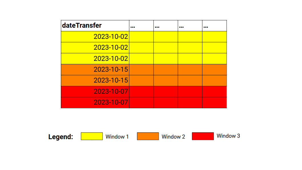
Now, lets create a window object using the transf DataFrame as our target. This DataFrame describes a set of transfers made in a fictitious bank. So a reasonable way of splitting this DataFrame is by day. That means that we can split this DataFrame into groups (or ranges) of rows by using the dateTransfer column. As a result, each partition in the dateTransfer column will create/identify a different window in this DataFrame.
window_spec = Window.partitionBy('dateTransfer')The above window object specifies that each unique value present in the dateTransfer column identifies a different window frame in the transf DataFrame. Figure 12.1 presents this idea visually. So each partition in the dateTransfer column creates a different window frame. And each window frame will become an input to a window function (when we use one).
Until this point, defining windows are very much like defining groups in your DataFrame with group by functions (i.e. windows are very similar to groups). But in the above example, we specified only the partition component of the windows. The partitioning component of the window object specifies which partitions of the DataFrame are translated into windows. In the other hand, the ordering component of the window object specifies how the rows within the window are ordered.
Defining the ordering component becomes very important when we are working with window functions that outputs (or that uses) indexes. As an example, you might want to use in your calculations the first (or the nth) row in each window. In a situation like this, the order in which these rows are founded inside the window affects directly the output of your window function. That is why the ordering component matters.
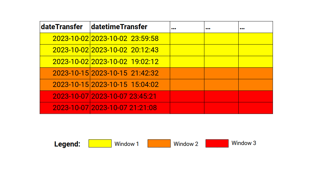
For example, we can say that the rows within each window should be in descending order according to the datetimeTransfer column:
from pyspark.sql.functions import col
window_spec = Window\
    .partitionBy('dateTransfer')\
    .orderBy(col('datetimeTransfer').desc())
With the above snippet, we are not only specifying how the window frames in the DataFrame are created (with the partitionBy()), but we are also specifying how the rows within the window are sorted (with the orderBy()). If we update our representation with the above window specification, we get something similar to Figure 12.2:
Is worth mentioning that, both partitionBy() and orderBy() methods accepts multiple columns as input. In other words, you can use a combination of columns both to define how the windows in your DataFrame will be created, and how the rows within these windows will be sorted.
As an example, the window specification below is saying: 1) that a window frame is created for each unique combination of dateTransfer and clientNumber; 2) that the rows within each window are ordered accordingly to transferCurrency (ascending order) and datetimeTransfer (descending order).
window_spec = Window\
    .partitionBy('dateTransfer', 'clientNumber')\
    .orderBy(
        col('transferCurrency').asc(),
        col('datetimeTransfer').desc()
    )
12.1.1 Partitioning or ordering or none
Is worth mentioning that both partioning and ordering components of the window specification are optional. You can create a window object that contains only a partioning component defined, or, only a ordering component, or, in fact, a window object that basically have neither of them defined.
As an example, all three objects below (w1, w2 and w3) are valid window objects. w1 have only the partition component defined, while w2 have only the ordering component defined. However, w3 have basically none of them defined, because w3 is partitioned by nothing. In a situation like this, a single window is created, and this window covers the entire DataFrame. It covers all the rows at once. Is like you were not using any window at all.
w1 = Window.partitionBy('x')
w2 = Window.orderBy('x')
w3 = Window.partitionBy()
So just be aware of this. Be aware that you can cover the entire DataFrame into a single window. Be aware that if you use a window object with neither components defined (Window.partitionBy()) your window function basically works with the entire DataFrame at once. In essence, this window function becomes similar to a normal aggregating function.
12.2 Introducing the over() clause
In order to use a window function you need to combine an over clause with a window object. If you pair these two components together, then, the function you are using becomes a window function.
Since we know now how to define window objects for our DataFrame, we can actually create and use this object to access window functionality, by pairing this window object with an over() clause.
In pyspark this over() clause is actually a method from the Column class. Since all aggregating functions available from the pyspark.sql.functions module produces a new Column object as output, we tend to use the over() method right after the function call.
For example, if we wanted to calculate the mean of x with the mean() function, and we had a window object called window_spec, we could use the mean() as a window function by writing mean(col('x')).over(window_spec).
from pyspark.sql.window import Window
from pyspark.sql.functions import mean, col
window_spec = Window\
    .partitionBy('y', 'z')\
    .orderBy('t')

mean(col('x')).over(window_spec)
If you see this over() method after a call of an aggregating function (such as sum(), mean(), etc.), then, you know that this aggregating function is being called as a window function.
The over() clause is also available in Spark SQL as the SQL keyword OVER. This means that you can use window functions in Spark SQL as well. But in Spark SQL, you write the window specification inside parentheses after the OVER keyword, and you specify each component with PARTITION BY AND ORDER BY keywords. We could replicate the above example in Spark SQL like this:
SELECT mean(x) OVER (PARTITION BY y, z ORDER BY t ASC)12.3 Window functions vs group by functions
Despite their similarities, window functions and group by functions are used for different purposes. One big difference between them, is that when you use groupby() + agg() you get one output row per each input group of rows, but in contrast, a window function outputs one row per input row. In other words, for a window of \(n\) input rows a window function outputs \(n\) rows that contains the same result (or the same aggregate result).
For example, lets suppose you want to calculate the total value transfered within each day. If you use a groupby() + agg() strategy, you get as result a new DataFrame containing one row for each unique date present in the dateTransfer column:
from pyspark.sql.functions import sum
transf\
    .orderBy('dateTransfer')\
    .groupBy('dateTransfer')\
    .agg(sum(col('transferValue')).alias('dayTotalTransferValue'))\
    .show(5)
+------------+---------------------+
|dateTransfer|dayTotalTransferValue|
+------------+---------------------+
| 2022-01-01| 39630.7|
| 2022-01-02| 70031.46|
| 2022-01-03| 50957.869999999995|
| 2022-01-04| 56068.34|
| 2022-01-05| 47082.04|
+------------+---------------------+
only showing top 5 rows
On the other site, if you use sum() as a window function instead, you get as result one row for each transfer. That is, you get one row of output for each input row in the transf DataFrame. The value that is present in the new column created (dayTotalTransferValue) is the total value transfered for the window (or the range of rows) that corresponds to the date in the dateTransfer column.
In other words, the value 39630.7 below corresponds to the sum of the transferValue column when dateTransfer == "2022-01-01":
window_spec = Window.partitionBy('dateTransfer')
transf\
    .select('dateTransfer', 'transferID', 'transferValue')\
    .withColumn(
        'dayTotalTransferValue',
        sum(col('transferValue')).over(window_spec)
    )\
    .show(5)
+------------+----------+-------------+---------------------+
|dateTransfer|transferID|transferValue|dayTotalTransferValue|
+------------+----------+-------------+---------------------+
| 2022-01-01| 20221148| 5547.13| 39630.7|
| 2022-01-01| 20221147| 9941.0| 39630.7|
| 2022-01-01| 20221146| 5419.9| 39630.7|
| 2022-01-01| 20221145| 5006.0| 39630.7|
| 2022-01-01| 20221144| 8640.06| 39630.7|
+------------+----------+-------------+---------------------+
only showing top 5 rows
You probably already seen this pattern in other data frameworks. As a quick comparison, if you were using the tidyverse framework, you could calculate the exact same result above with the following snippet of R code:
transf |>
    group_by(dateTransfer) |>
    mutate(
        dayTotalTransferValue = sum(transferValue)
    )
In contrast, you would need the following snippet of Python code to get the same result in the pandas framework:
transf['dayTotalTransferValue'] = transf['transferValue']\
    .groupby(transf['dateTransfer'])\
    .transform('sum')
12.4 Ranking window functions
The functions row_number(), rank() and dense_rank() from the pyspark.sql.functions module are ranking functions, in the sense that they seek to rank each row in the input window according to a ranking system. These functions are identical to their peers in MySQL4 ROW_NUMBER(), RANK() and DENSE_RANK().
The function row_number() simply returns a unique and sequential number to each row in a window, starting from 1. It is a quick way of marking each row with an unique and sequential number.
from pyspark.sql.functions import row_number
window_spec = Window\
    .partitionBy('dateTransfer')\
    .orderBy('datetimeTransfer')

transf\
    .select(
        'dateTransfer',
        'datetimeTransfer',
        'transferID'
    )\
    .withColumn('rowID', row_number().over(window_spec))\
    .show(5)
+------------+-------------------+----------+-----+
|dateTransfer| datetimeTransfer|transferID|rowID|
+------------+-------------------+----------+-----+
| 2022-01-01|2022-01-01 03:56:58| 20221143| 1|
| 2022-01-01|2022-01-01 04:07:44| 20221144| 2|
| 2022-01-01|2022-01-01 09:00:18| 20221145| 3|
| 2022-01-01|2022-01-01 10:17:04| 20221146| 4|
| 2022-01-01|2022-01-01 16:14:30| 20221147| 5|
+------------+-------------------+----------+-----+
only showing top 5 rows
The row_number() function is also very useful when you are trying to collect the rows in each window that contains the smallest or biggest value in the window. If the ordering of your window specification is in ascending order, then, the first row in the window will contain the smallest value in the current window. In contrast, if the ordering is in descending order, then, the first row in the window will contain the biggest value in the current window.
This is interesting, because lets suppose you wanted to find the rows that contained the maximum transfer values in each day. A groupby() + agg() strategy would tell you which are the maximum transfer values in each day. But it would not tell you where are the rows in the DataFrame that contains these maximum values. A Window object + row_number() + filter() can help you to get this answer.
window_spec = Window\
    .partitionBy('dateTransfer')\
    .orderBy(col('transferValue').desc())

# The row with rowID == 1 is the first row in each window
transf\
    .withColumn('rowID', row_number().over(window_spec))\
    .filter(col('rowID') == 1)\
    .select(
        'dateTransfer', 'rowID',
        'transferID', 'transferValue'
    )\
    .show(5)
+------------+-----+----------+-------------+
|dateTransfer|rowID|transferID|transferValue|
+------------+-----+----------+-------------+
| 2022-01-01| 1| 20221147| 9941.0|
| 2022-01-02| 1| 20221157| 10855.01|
| 2022-01-03| 1| 20221165| 8705.65|
| 2022-01-04| 1| 20221172| 9051.0|
| 2022-01-05| 1| 20221179| 9606.0|
+------------+-----+----------+-------------+
only showing top 5 rows
The rank() and dense_rank() functions are similar to each other. They both rank the rows with integers, just like row_number(). But if there is a tie between two rows (that means that both rows have the same value in the ordering column, so it becomes a tie, we do not know which one of these rows should come first), then, these functions will repeat the same number/index for these rows in tie. Lets use the df below as a quick example:
data = [
    (1, 3000), (1, 2400),
    (1, 4200), (1, 4200),
    (2, 1500), (2, 2000),
    (2, 3000), (2, 3000),
    (2, 4500), (2, 4600)
]
df = spark.createDataFrame(data, ['id', 'value'])
If we apply both rank() and dense_rank() over this DataFrame with the same window specification, we can see the difference between these functions. In essence, rank() leave gaps in the indexes that come right after any tied rows, while dense_rank() does not.
from pyspark.sql.functions import rank, dense_rank
window_spec = Window\
    .partitionBy('id')\
    .orderBy('value')

# With rank() there are gaps in the indexes
df.withColumn('with_rank', rank().over(window_spec))\
    .show()
[Stage 14:> (0 + 12) / 12]+---+-----+---------+
| id|value|with_rank|
+---+-----+---------+
| 1| 2400| 1|
| 1| 3000| 2|
| 1| 4200| 3|
| 1| 4200| 3|
| 2| 1500| 1|
| 2| 2000| 2|
| 2| 3000| 3|
| 2| 3000| 3|
| 2| 4500| 5|
| 2| 4600| 6|
+---+-----+---------+
# With dense_rank() there are no gaps in the indexes
df.withColumn('with_dense_rank', dense_rank().over(window_spec))\
    .show()
+---+-----+---------------+
| id|value|with_dense_rank|
+---+-----+---------------+
| 1| 2400| 1|
| 1| 3000| 2|
| 1| 4200| 3|
| 1| 4200| 3|
| 2| 1500| 1|
| 2| 2000| 2|
| 2| 3000| 3|
| 2| 3000| 3|
| 2| 4500| 4|
| 2| 4600| 5|
+---+-----+---------------+
12.5 Agreggating window functions
In essence, all agreggating functions from the pyspark.sql.functions module (like sum(), mean(), count(), max() and min()) can be used as a window function. So you can apply any agreggating function as a window function. You just need to use the over() clause with a Window object.
We could for example see how much each transferValue deviates from the daily mean of transfered value. This might be a valuable information in case you are planning to do some statistical inference over this data. Here is an example of what this would looks like in pyspark:
from pyspark.sql.functions import mean
window_spec = Window.partitionBy('dateTransfer')

mean_deviation_expr = (
    col('transferValue')
    - mean(col('transferValue')).over(window_spec)
)

transf\
    .select('dateTransfer', 'transferValue')\
    .withColumn('meanDeviation', mean_deviation_expr)\
    .show(5)
+------------+-------------+-------------------+
|dateTransfer|transferValue| meanDeviation|
+------------+-------------+-------------------+
| 2022-01-01| 5547.13|-1057.9866666666658|
| 2022-01-01| 9941.0| 3335.883333333334|
| 2022-01-01| 5419.9|-1185.2166666666662|
| 2022-01-01| 5006.0|-1599.1166666666659|
| 2022-01-01| 8640.06| 2034.9433333333336|
+------------+-------------+-------------------+
only showing top 5 rows
As another example, you might want to calculate how much a specific transfer value represents of represents of the total amount transferred daily. You could just get the total amount transferred daily by applying the sum() function over windows partitioned by dateTransfer. Then, you just need to divide the current transferValue by the result of this sum() function, and you get the proportion you are looking for.
from pyspark.sql.functions import sum
proportion_expr = (
    col('transferValue')
    / sum(col('transferValue')).over(window_spec)
)

transf\
    .select('dateTransfer', 'transferValue')\
    .withColumn('proportionDailyTotal', proportion_expr)\
    .show(5)
+------------+-------------+--------------------+
|dateTransfer|transferValue|proportionDailyTotal|
+------------+-------------+--------------------+
| 2022-01-01| 5547.13| 0.1399705278988259|
| 2022-01-01| 9941.0| 0.25084088850310493|
| 2022-01-01| 5419.9| 0.1367601379738435|
| 2022-01-01| 5006.0| 0.1263162144499088|
| 2022-01-01| 8640.06| 0.2180143171833957|
+------------+-------------+--------------------+
only showing top 5 rows
12.6 Getting the next and previous row with lead() and lag()
There is one pair functions that is worth talking about in this chapter, which are lead() and lag(). These functions are very useful in the context of windows, because they return the value in the next and previous rows considering your current position in your DataFrame.
These functions basically performs the same operation as their peers dplyr::lead() and dplyr::lag()5 from the tidyverse framework. In essence, lead() will return the value of the next row, while lag() will return the value of the previous row.
from pyspark.sql.functions import lag, lead
window_spec = Window\
    .partitionBy('dateTransfer')\
    .orderBy('datetimeTransfer')

lead_expr = lead('transferValue').over(window_spec)
lag_expr = lag('transferValue').over(window_spec)

transf\
    .withColumn('nextValue', lead_expr)\
    .withColumn('previousValue', lag_expr)\
    .select(
        'datetimeTransfer',
        'transferValue',
        'nextValue',
        'previousValue'
    )\
    .show(5)
+-------------------+-------------+---------+-------------+
| datetimeTransfer|transferValue|nextValue|previousValue|
+-------------------+-------------+---------+-------------+
|2022-01-01 03:56:58| 5076.61| 8640.06| NULL|
|2022-01-01 04:07:44| 8640.06| 5006.0| 5076.61|
|2022-01-01 09:00:18| 5006.0| 5419.9| 8640.06|
|2022-01-01 10:17:04| 5419.9| 9941.0| 5006.0|
|2022-01-01 16:14:30| 9941.0| 5547.13| 5419.9|
+-------------------+-------------+---------+-------------+
only showing top 5 rows