sql_query = '''
SELECT *
FROM (
  VALUES (11), (31), (24), (35)
) AS List(Codes)
'''
spark.sql(sql_query).show()+-----+
|Codes|
+-----+
| 11|
| 31|
| 24|
| 35|
+-----+
pysparkAs we discussed in Chapter 2, Spark is a multi-language engine for large-scale data processing. This means that we can build our Spark application using many different languages (like Java, Scala, Python and R). Furthermore, you can also use the Spark SQL module of Spark to translate all of your transformations into pure SQL queries.
In more details, Spark SQL is a Spark module for structured data processing (Apache Spark Official Documentation 2022). Because this module works with Spark DataFrames, using SQL, you can translate all transformations that you build with the DataFrame API into a SQL query.
Therefore, you can mix python code with SQL queries very easily in Spark. Virtually all transformations exposed in python throughout this book, can be translated into a SQL query using this module of Spark. We will focus a lot on this exchange between Python and SQL in this chapter.
However, this also means that the Spark SQL module does not handle the transformations produced by the unstructured APIs of Spark, i.e. the Dataset API. Since the Dataset API is not available in pyspark, it is not covered in this book.
sql() method as the main entrypointThe main entrypoint, that is, the main bridge that connects Spark SQL to Python is the sql() method of your Spark Session. This method accepts a SQL query inside a string as input, and will always output a new Spark DataFrame as result. That is why I used the show() method right after sql(), in the example below, to see what this new Spark DataFrame looked like.
As a first example, lets look at a very basic SQL query, that just select a list of code values:
SELECT *
FROM (
VALUES (11), (31), (24), (35)
) AS List(Codes)To run the above SQL query, and see its results, I must write this query into a string, and give this string to the sql() method of my Spark Session. Then, I use the show() action to see the actual result rows of data generated by this query:
sql_query = '''
SELECT *
FROM (
  VALUES (11), (31), (24), (35)
) AS List(Codes)
'''

spark.sql(sql_query).show()
+-----+
|Codes|
+-----+
| 11|
| 31|
| 24|
| 35|
+-----+
If you want to execute a very short SQL query, is fine to write it inside a single pair of quotation marks (for example "SELECT * FROM sales.per_day"). However, since SQL queries usually take multiple lines, you can write your SQL query inside a python docstring (created by a pair of three quotation marks), like in the example above.
Having this in mind, every time you want to execute a SQL query, you can use this sql() method from the object that holds your Spark Session. So the sql() method is the bridge between pyspark and SQL. You give it a pure SQL query inside a string, and, Spark will execute it, considering your Spark SQL context.
Is worth pointing out that, although being the main bridge between Python and SQL, the Spark Session sql() method can execute only a single SQL statement per run. This means that if you try to execute two sequential SQL statements at the same time with sql(), then, Spark SQL will automatically raise a ParseException error, which usually complains about an “extra input”.
In the example below, we are doing two very basic steps to SQL. We first create a dummy database with a CREATE DATABASE statement, then, we ask SQL to use this new database that we created as the default database of the current session, with a USE statement.
CREATE DATABASE `dummy`;
USE `dummy`;
If we try to execute these two steps at once, by using the sql() method, Spark complains with a ParseException, indicating that we have a sytax error in our query, like in the example below:
query = '''
CREATE DATABASE `dummy`;
USE `dummy`;
'''

spark.sql(query).show()
Traceback (most recent call last):
File "<stdin>", line 1, in <module>
File "/opt/spark/python/pyspark/sql/session.py", line 1034, in sql
return DataFrame(self._jsparkSession.sql(sqlQuery), self)
File "/opt/spark/python/lib/py4j-0.10.9.5-src.zip/py4j/java_gateway.py", line 1321, in __call__
File "/opt/spark/python/pyspark/sql/utils.py", line 196, in deco
raise converted from None
pyspark.sql.utils.ParseException:
Syntax error at or near 'USE': extra input 'USE'(line 3, pos 0)
== SQL ==
CREATE DATABASE `dummy`;
USE `dummy`;
^^^However, there is nothing wrong about the above SQL statements. They are both correct and valid SQL statements, both semantically and syntactically. In other words, the case above results in a ParseException error solely because it contains two different SQL statements.
In essence, the spark.sql() method always expect a single SQL statement as input, and, therefore, it will try to parse this input query as a single SQL statement. If it finds multiple SQL statements inside this input string, the method will automatically raise the above error.
Now, be aware that some SQL queries can take multiple lines, but, still be considered a single SQL statement. A query started by a WITH clause is usually a good example of a SQL query that can group multiple SELECT statements, but still be considered a single SQL statement as a whole:
-- The query below would execute
-- perfectly fine inside spark.sql():
WITH table1 AS (
  SELECT *
  FROM somewhere
),

filtering AS (
  SELECT *
  FROM table1
  WHERE dateOfTransaction == CAST("2022-02-02" AS DATE)
)

SELECT *
FROM filtering
Another example of a usually big and complex query, that can take multiple lines but still be considered a single SQL statement, is a single SELECT statement that selects multiple subqueries that are nested together, like this:
-- The query below would also execute
-- perfectly fine inside spark.sql():
SELECT *
FROM (
  -- First subquery.
  SELECT *
  FROM (
    -- Second subquery..
    SELECT *
    FROM (
      -- Third subquery...
      SELECT *
      FROM (
        -- Ok this is enough....
      )
    )
  )
)
However, if we had multiple separate SELECT statements that were independent on each other, like in the example below, then, spark.sql() would issue an ParseException error if we tried to execute these three SELECT statements inside the same input string.
-- These three statements CANNOT be executed
-- at the same time inside spark.sql()
SELECT * FROM something;
SELECT * FROM somewhere;
SELECT * FROM sometime;
As a conclusion, if you want to easily execute multiple statements, you can use a for loop which calls spark.sql() for each single SQL statement:
statements = '''SELECT * FROM something;
SELECT * FROM somewhere;
SELECT * FROM sometime;'''

statements = statements.split('\n')
for statement in statements:
spark.sql(statement)In real life jobs at the industry, is very likely that your data will be allocated inside a SQL-like database. Spark can connect to a external SQL database through JDBC/ODBC connections, or, read tables from Apache Hive. This way, you can sent your SQL queries to this external database.
However, to expose more simplified examples throughout this chapter, we will use pyspark to create a simple temporary SQL table in our Spark SQL context, and use this temporary SQL table in our examples of SQL queries. This way, we avoid the work to connect to some existing SQL database, and, still get to learn how to use SQL queries in pyspark.
First, lets create our Spark Session. You can see below that I used the config() method to set a specific option of the session called catalogImplementation to the value "hive". This option controls the implementation of the Spark SQL Catalog, which is a core part of the SQL functionality of Spark 1.
Spark usually complain with a AnalysisException error when you try to create SQL tables with this option undefined (or not configured). So, if you decide to follow the examples of this chapter, please always set this option right at the start of your script2.
from pyspark.sql import SparkSession
spark = SparkSession\
  .builder\
  .config("spark.sql.catalogImplementation","hive")\
.getOrCreate()TABLEs versus VIEWsTo run a complete SQL query over any Spark DataFrame, you must register this DataFrame in the Spark SQL Catalog of your Spark Session. You can register a Spark DataFrame into this catalog as a physical SQL TABLE, or, as a SQL VIEW.
If you are familiar with the SQL language and Relational DataBase Management Systems - RDBMS (such as MySQL), you probably already heard of these two types (TABLE or VIEW) of SQL objects. But if not, we will explain each one in this section. Is worth pointing out that choosing between these two types does not affect your code, or your transformations in any way. It just affect the way that Spark SQL stores the table/DataFrame itself.
VIEWs are stored as SQL queries or memory pointersWhen you register a DataFrame as a SQL VIEW, the query to produce this DataFrame is stored, not the DataFrame itself. There are also cases where Spark store a memory pointer instead, that points to the memory adress where this DataFrame is stored in memory. In this perspective, Spark SQL use this pointer every time it needs to access this DataFrame.
Therefore, when you call (or access) this SQL VIEW inside your SQL queries (for example, with a SELECT * FROM statement), Spark SQL will automatically get this SQL VIEW “on the fly” (or “on runtime”), by executing the query necessary to build the initial DataFrame that you stored inside this VIEW, or, if this DataFrame is already stored in memory, Spark will look at the specific memory address it is stored.
In other words, when you create a SQL VIEW, Spark SQL do not store any physical data or rows of the DataFrame. It just stores the SQL query necessary to build your DataFrame. In some way, you can interpret any SQL VIEW as an abbreviation to a SQL query, or a “nickname” to an already existing DataFrame.
As a consequence, for most “use case scenarios”, SQL VIEWs are easier to manage inside your data pipelines. Because you usually do not have to update them. Since they are calculated from scratch, at the moment you request for them, a SQL VIEW will always translate the most recent version of the data.
This means that the concept of a VIEW in Spark SQL is very similar to the concept of a VIEW in other types of SQL databases, such as the MySQL database. If you read the official documentation for the CREATE VIEW statement at MySQL3 you will get a similar idea of a VIEW:
The select_statement is a SELECT statement that provides the definition of the view. (Selecting from the view selects, in effect, using the SELECT statement.) …
The above statement, tells us that selecing a VIEW causes the SQL engine to execute the expression defined at select_statement using the SELECT statement. In other words, in MySQL, a SQL VIEW is basically an alias to an existing SELECT statement.
VIEWsAlthough a Spark SQL VIEW being very similar to other types of SQL VIEW (such as the MySQL type), on Spark applications, SQL VIEWs are usually registered as TEMPORARY VIEWs4 instead of standard (and “persistent”) SQL VIEW as in MySQL.
At MySQL there is no notion of a “temporary view”, although other popular kinds of SQL databases do have it, such as the PostGreSQL database5. So, a temporary view is not a exclusive concept of Spark SQL. However, is a special type of SQL VIEW that is not present in all popular kinds of SQL databases.
In other words, both Spark SQL and MySQL support the CREATE VIEW statement. In contrast, statements such as CREATE TEMPORARY VIEW and CREATE OR REPLACE TEMPORARY VIEW are available in Spark SQL, but not in MySQL.
VIEW in the Spark SQL CatalogIn pyspark, you can register a Spark DataFrame as a temporary SQL VIEW with the createTempView() or createOrReplaceTempView() DataFrame methods. These methods are equivalent to CREATE TEMPORARY VIEW and CREATE OR REPLACE TEMPORARY VIEW SQL statements of Spark SQL, respectively.
In essence, these methods register your Spark DataFrame as a temporary SQL VIEW, and have a single input, which is the name you want to give to this new SQL VIEW you are creating inside a string:
# To save the `df` DataFrame as a SQL VIEW,
# use one of the methods below:
df.createTempView('example_view')
df.createOrReplaceTempView('example_view')
After we executed the above statements, we can now access and use the df DataFrame in any SQL query, like in the example below:
sql_query = '''
SELECT *
FROM example_view
WHERE value > 20
'''

spark.sql(sql_query).show()
[Stage 0:> (0 + 1) / 1] +---+-----+----------+
| id|value| date|
+---+-----+----------+
| 1| 28.3|2021-01-01|
| 3| 20.1|2021-01-02|
+---+-----+----------+
So you use the createTempView() or createOrReplaceTempView() methods when you want to make a Spark DataFrame created in pyspark (that is, a python object), available to Spark SQL.
Besides that, you also have the option to create a temporary VIEW by using pure SQL statements trough the sql() method. However, when you create a temporary VIEW using pure SQL, you can only use (inside this VIEW) native SQL objects that are already stored inside your Spark SQL Context.
This means that you cannot make a Spark DataFrame created in python available to Spark SQL, by using a pure SQL inside the sql() method. To do this, you have to use the DataFrame methods createTempView() and createOrReplaceTempView().
As an example, the query below uses pure SQL statements to creates the active_brazilian_users temporary VIEW, which selects an existing SQL table called hubspot.user_mails:
CREATE TEMPORARY VIEW active_brazilian_users AS
SELECT *
FROM hubspot.user_mails
WHERE state == 'Active'
AND country_location == 'Brazil'
Temporary VIEWs like the one above (which are created from pure SQL statements being executed inside the sql() method) are kind of unusual in Spark SQL. Because you can easily avoid the work of creating a VIEW by using Common Table Expression (CTE) on a WITH statement, like in the query below:
WITH active_brazilian_users AS (
  SELECT *
  FROM hubspot.user_mails
  WHERE state == 'Active'
  AND country_location == 'Brazil'
)

SELECT A.user, SUM(sale_value), B.user_email
FROM sales.sales_per_user AS A
INNER JOIN active_brazilian_users AS B
GROUP BY A.user, B.user_email
Just as a another example, you can also run a SQL query that creates a persistent SQL VIEW (that is, without the TEMPORARY clause). In the example below, I am saving the simple query that I showed at the beginning of this chapter inside a VIEW called list_of_codes. This CREATE VIEW statement, register a persistent SQL VIEW in the SQL Catalog.
sql_query = '''
CREATE OR REPLACE VIEW list_of_codes AS
SELECT *
FROM (
  VALUES (11), (31), (24), (35)
) AS List(Codes)
'''

spark.sql(sql_query)DataFrame[]Now, every time I want to use this SQL query that selects a list of codes, I can use this list_of_codes as a shortcut:
spark.sql("SELECT * FROM list_of_codes").show()+-----+
|Codes|
+-----+
| 11|
| 31|
| 24|
| 35|
+-----+
TABLEs are stored as physical tablesIn the other hand, SQL TABLEs are the “opposite” of SQL VIEWs. That is, SQL TABLEs are stored as physical tables inside the SQL database. In other words, each one of the rows of your table are stored inside the SQL database.
Because of this characteristic, when dealing with huges amounts of data, SQL TABLEs are usually faster to load and transform. Because you just have to read the data stored on the database, you do not need to calculate it from scratch every time you use it.
But, as a collateral effect, you usually have to physically update the data inside this TABLE, by using, for example, INSERT INTO statements. In other words, when dealing with SQL TABLE’s you usually need to create (and manage) data pipelines that are responsible for periodically update and append new data to this SQL TABLE, and this might be a big burden to your process.
TABLEs in the Spark SQL CatalogIn pyspark, you can register a Spark DataFrame as a SQL TABLE with the write.saveAsTable() DataFrame method. This method accepts, as first input, the name you want to give to this SQL TABLE inside a string.
# To save the `df` DataFrame as a SQL TABLE:
df.write.saveAsTable('example_table')
As you expect, after we registered the DataFrame as a SQL table, we can now run any SQL query over example_table, like in the example below:
spark.sql("SELECT SUM(value) FROM example_table").show()+----------+
|sum(value)|
+----------+
| 76.8|
+----------+You can also use pure SQL queries to create an empty SQL TABLE from scratch, and then, feed this table with data by using INSERT INTO statements. In the example below, we create a new database called examples, and, inside of it, a table called code_brazil_states. Then, we use multiple INSERT INTO statements to populate this table with few rows of data.
all_statements = '''CREATE DATABASE `examples`;
USE `examples`;
CREATE TABLE `code_brazil_states` (`code` INT, `state_name` STRING);
INSERT INTO `code_brazil_states` VALUES (31, "Minas Gerais");
INSERT INTO `code_brazil_states` VALUES (15, "Pará");
INSERT INTO `code_brazil_states` VALUES (41, "Paraná");
INSERT INTO `code_brazil_states` VALUES (25, "Paraíba");'''

statements = all_statements.split('\n')
for statement in statements:
  spark.sql(statement)
We can see now this new physical SQL table using a simple query like this:
spark\
  .sql('SELECT * FROM examples.code_brazil_states')\
  .show()
+----+------------+
|code| state_name|
+----+------------+
| 41| Paraná|
| 31|Minas Gerais|
| 15| Pará|
| 25| Paraíba|
+----+------------+There are other arguments that you might want to use in the write.saveAsTable() method, like the mode argument. This argument controls how Spark will save your data into the database. By default, write.saveAsTable() uses the mode = "error" by default. In this mode, Spark will look if the table you referenced already exists, before it saves your data.
Let’s get back to the code we showed before (which is reproduced below). In this code, we asked Spark to save our data into a table called "example_table". Spark will look if a table with this name already exists. If it does, then, Spark will raise an error that will stop the process (i.e. no data is saved).
df.write.saveAsTable('example_table')Raising an error when you do not want to accidentaly affect a SQL table that already exist, is a good practice. But, you might want to not raise an error in this situation. In case like this, you might want to just ignore the operation, and get on with your life. For cases like this, write.saveAsTable() offers the mode = "ignore".
So, in the code example below, we are trying to save the df DataFrame into a table called example_table. But if this example_table already exist, Spark will just silently ignore this operation, and will not save any data.
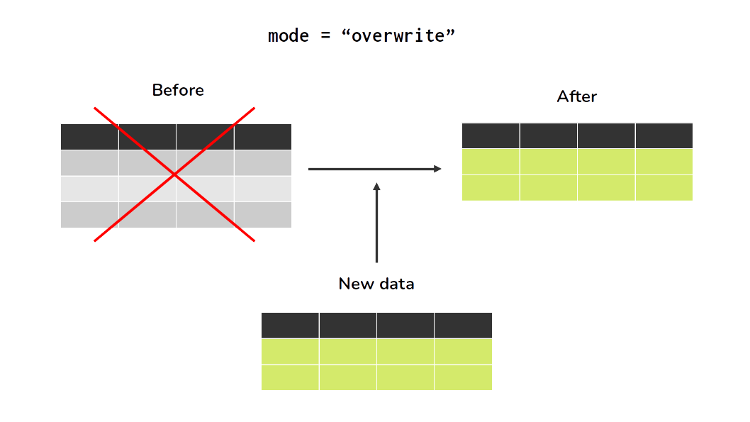
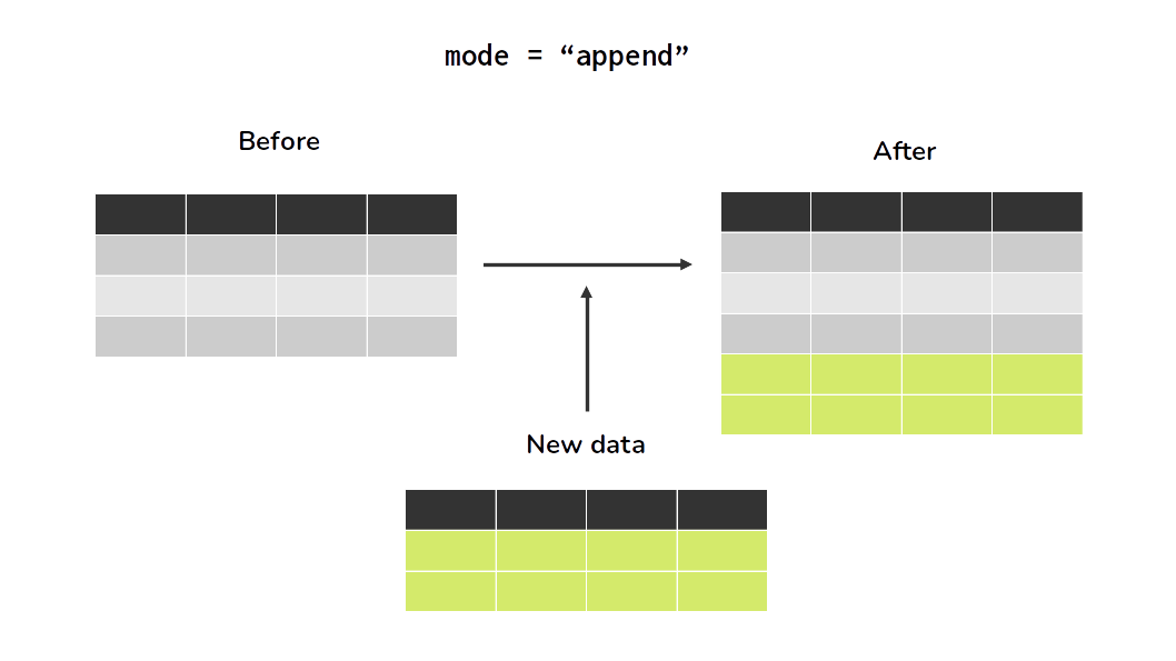
df.write.saveAsTable('example_table', mode = "ignore")In addition, write.saveAsTable() offers two more different modes, which are mode = "overwrite" and mode = "append". When you use one these two modes, Spark will always save your data, no matter if the SQL table you are trying to save into already exist or not. In essence, these two modes control whether Spark will delete or keep previous rows of the SQL table intact, before it saves any new data.
When you use mode = "overwrite", Spark will automatically rewrite/replace the entire table with the current data of your DataFrame. In contrast, when you use mode = "append", Spark will just append (or insert, or add) this data into the table. The subfigures at Figure 7.1 demonstrates these two modes visually.
You can see the full list of arguments of write.SaveAsTable(), and their description by looking at the documentation6.
When you register any Spark DataFrame as a SQL TABLE, it becomes a persistent source. Because the contents, the data, the rows of the table are stored on disk, inside a database, and can be accessed any time, even after you close or restart your computer (or your Spark Session). In other words, it becomes “persistent” as in the sense of “it does not die”.
As another example, when you save a specific SQL query as a SQL VIEW with the CREATE VIEW statement, this SQL VIEW is saved inside the database. As a consequence, it becomes a persistent source as well, and can be accessed and reused in other Spark Sessions, unless you explicit drop (or “remove”) this SQL VIEW with a DROP VIEW statement.
However, with methods like createTempView() and createOrReplaceTempView() you register your Spark DataFrame as a temporary SQL VIEW. This means that the life (or time of existence) of this VIEW is tied to your Spark Session. In other words, it will exist in your Spark SQL Catalog only for the duration of your Spark Session. When you close your Spark Session, this VIEW just dies. When you start a new Spark Session it does not exist anymore. As a result, you have to register your DataFrame again at the catalog to use it one more time.
pysparkRemember, to run SQL queries over any Spark DataFrame, you must register this DataFrame into the Spark SQL Catalog. Because of it, this Spark SQL Catalog works almost as the bridge that connects the python objects that hold your Spark DataFrames to the Spark SQL context. Without it, Spark SQL will not find your Spark DataFrames. As a result, it can not run any SQL query over it.
When you try to use a DataFrame that is not currently registered at the Spark SQL Catalog, Spark will automatically raise a AnalysisException, like in the example below:
spark\
  .sql("SELECT * FROM this.does_not_exist")\
  .show()
AnalysisException: Table or view not foundThe methods saveAsTable(), createTempView() and createOrReplaceTempView() are the main methods to register your Spark DataFrame into this Spark SQL Catalog. This means that you have to use one of these methods before you run any SQL query over your Spark DataFrame.
penguins DataFrameOver the next examples in this chapter, we will explore the penguins DataFrame. This is the penguins dataset from the palmerpenguins R library7. It stores data of multiple measurements of penguin species from the islands in Palmer Archipelago.
These measurements include size (flipper length, body mass, bill dimensions) and sex, and they were collected by researchers of the Antarctica LTER program, a member of the Long Term Ecological Research Network. If you want to understand more about each field/column present in this dataset, I recommend you to read the official documentation of this dataset8.
To get this data, you can download the CSV file called penguins.csv (remember that this CSV can be downloaded from the book repository9). In the code below, I am reading this CSV file and creating a Spark DataFrame with its data. Then, I register this Spark DataFrame as a SQL temporary view (called penguins_view) using the createOrReplaceTempView() method.
path = "../Data/penguins.csv"
penguins = spark.read\
  .csv(path, header = True)

penguins.createOrReplaceTempView('penguins_view')
After these commands, I have now a SQL view called penguins_view registered in my Spark SQL context, which I can query it, using pure SQL:
spark.sql('SELECT * FROM penguins_view').show(5)+-------+---------+--------------+-------------+-----------------+-----------+------+----+
|species| island|bill_length_mm|bill_depth_mm|flipper_length_mm|body_mass_g| sex|year|
+-------+---------+--------------+-------------+-----------------+-----------+------+----+
| Adelie|Torgersen| 39.1| 18.7| 181| 3750| male|2007|
| Adelie|Torgersen| 39.5| 17.4| 186| 3800|female|2007|
| Adelie|Torgersen| 40.3| 18| 195| 3250|female|2007|
| Adelie|Torgersen| NULL| NULL| NULL| NULL| NULL|2007|
| Adelie|Torgersen| 36.7| 19.3| 193| 3450|female|2007|
+-------+---------+--------------+-------------+-----------------+-----------+------+----+
only showing top 5 rows
An obvious way to access any SQL TABLE or VIEW registered in your Spark SQL context, is to select it, through a simple SELECT * FROM statement, like we saw in the previous examples. However, it can be quite annoying to type “SELECT * FROM” every time you want to use a SQL TABLE or VIEW in Spark SQL.
That is why Spark offers a shortcut to us, which is the table() method of your Spark session. In other words, the code spark.table("table_name") is a shortcut to spark.sql("SELECT * FROM table_name"). They both mean the same thing. For example, we could access penguins_view as:
spark\
  .table('penguins_view')\
  .show(5)
+-------+---------+--------------+-------------+-----------------+-----------+------+----+
|species| island|bill_length_mm|bill_depth_mm|flipper_length_mm|body_mass_g| sex|year|
+-------+---------+--------------+-------------+-----------------+-----------+------+----+
| Adelie|Torgersen| 39.1| 18.7| 181| 3750| male|2007|
| Adelie|Torgersen| 39.5| 17.4| 186| 3800|female|2007|
| Adelie|Torgersen| 40.3| 18| 195| 3250|female|2007|
| Adelie|Torgersen| NULL| NULL| NULL| NULL| NULL|2007|
| Adelie|Torgersen| 36.7| 19.3| 193| 3450|female|2007|
+-------+---------+--------------+-------------+-----------------+-----------+------+----+
only showing top 5 rows
As I noted at Section 4.2, columns of a Spark DataFrame (or objects of class Column) are closely related to expressions. As a result, you usually use and execute expressions in Spark when you want to transform (or mutate) columns of a Spark DataFrame.
This is no different for SQL expressions. A SQL expression is basically any expression you would use on the SELECT statement of your SQL query. As you can probably guess, since they are used in the SELECT statement, these expressions are used to transform columns of a Spark DataFrame.
There are many column transformations that are particularly verbose and expensive to write in “pure” pyspark. But you can use a SQL expression in your favor, to translate this transformation into a more short and concise form. Virtually any expression you write in pyspark can be translated into a SQL expression.
To execute a SQL expression, you give this expression inside a string to the expr() function from the pyspark.sql.functions module. Since expressions are used to transform columns, you normally use the expr() function inside a withColumn() or a select() DataFrame method, like in the example below:
from pyspark.sql.functions import expr

spark\
  .table('penguins_view')\
  .withColumn(
    'specie_island',
    expr("CONCAT(species, '_', island)")
  )\
  .withColumn(
    'sex_short',
    expr("CASE WHEN sex == 'male' THEN 'M' ELSE 'F' END")
  )\
  .select('specie_island', 'sex_short')\
  .show(5)
+----------------+---------+
| specie_island|sex_short|
+----------------+---------+
|Adelie_Torgersen| M|
|Adelie_Torgersen| F|
|Adelie_Torgersen| F|
|Adelie_Torgersen| F|
|Adelie_Torgersen| F|
+----------------+---------+
only showing top 5 rows
I particulaly like to write “if-else” or “case-when” statements using a pure CASE WHEN SQL statement inside the expr() function. By using this strategy you usually get a more simple statement that translates the intention of your code in a cleaner way. But if I wrote the exact same CASE WHEN statement above using pure pyspark functions, I would end up with a shorter (but “less clean”) statement using the when() and otherwise() functions:
from pyspark.sql.functions import (
  when, col,
  concat, lit
)

spark\
  .table('penguins_view')\
  .withColumn(
    'specie_island',
    concat('species', lit('_'), 'island')
  )\
  .withColumn(
    'sex_short',
    when(col("sex") == 'male', 'M')\
      .otherwise('F')
  )\
  .select('specie_island', 'sex_short')\
  .show(5)
+----------------+---------+
| specie_island|sex_short|
+----------------+---------+
|Adelie_Torgersen| M|
|Adelie_Torgersen| F|
|Adelie_Torgersen| F|
|Adelie_Torgersen| F|
|Adelie_Torgersen| F|
+----------------+---------+
only showing top 5 rows
All DataFrame API transformations that you write in Python (using pyspark) can be translated into SQL queries/expressions using the Spark SQL module. Since the DataFrame API is a core part of pyspark, the majority of python code you write with pyspark can be translated into SQL queries (if you wanto to).
Is worth pointing out, that, no matter which language you choose (Python or SQL), they are both further compiled to the same base instructions. The end result is that the Python code you write and his SQL translated version will perform the same (they have the same efficiency), because they are compiled to the same instructions before being executed by Spark.
When you translate the methods from the python DataFrame class (like orderBy(), select() and where()) into their equivalents in Spark SQL, you usually get SQL keywords (like ORDER BY, SELECT and WHERE).
For example, if I needed to get the top 5 penguins with the biggest body mass at penguins_view, that had sex equal to "female", and, ordered by bill length, I could run the following python code:
from pyspark.sql.functions import col
top_5 = penguins\
    .where(col('sex') == 'female')\
    .orderBy(col('body_mass_g').desc())\
    .limit(5)

top_5\
    .orderBy('bill_length_mm')\
    .show()
+-------+------+--------------+-------------+-----------------+-----------+------+----+
|species|island|bill_length_mm|bill_depth_mm|flipper_length_mm|body_mass_g| sex|year|
+-------+------+--------------+-------------+-----------------+-----------+------+----+
| Gentoo|Biscoe| 44.9| 13.3| 213| 5100|female|2008|
| Gentoo|Biscoe| 45.1| 14.5| 207| 5050|female|2007|
| Gentoo|Biscoe| 45.2| 14.8| 212| 5200|female|2009|
| Gentoo|Biscoe| 46.5| 14.8| 217| 5200|female|2008|
| Gentoo|Biscoe| 49.1| 14.8| 220| 5150|female|2008|
+-------+------+--------------+-------------+-----------------+-----------+------+----+
I could translate the above python code to the following SQL query:
WITH top_5 AS (
    SELECT *
    FROM penguins_view
    WHERE sex == 'female'
    ORDER BY body_mass_g DESC
    LIMIT 5
)

SELECT *
FROM top_5
ORDER BY bill_length_mm
Again, to execute the above SQL query inside pyspark we need to give this query as a string to the sql() method of our Spark Session, like this:
query = '''
WITH top_5 AS (
    SELECT *
    FROM penguins_view
    WHERE sex == 'female'
    ORDER BY body_mass_g DESC
    LIMIT 5
)

SELECT *
FROM top_5
ORDER BY bill_length_mm
'''

# The same result of the example above
spark.sql(query).show()
+-------+------+--------------+-------------+-----------------+-----------+------+----+
|species|island|bill_length_mm|bill_depth_mm|flipper_length_mm|body_mass_g| sex|year|
+-------+------+--------------+-------------+-----------------+-----------+------+----+
| Gentoo|Biscoe| 44.9| 13.3| 213| 5100|female|2008|
| Gentoo|Biscoe| 45.1| 14.5| 207| 5050|female|2007|
| Gentoo|Biscoe| 45.2| 14.8| 212| 5200|female|2009|
| Gentoo|Biscoe| 46.5| 14.8| 217| 5200|female|2008|
| Gentoo|Biscoe| 49.1| 14.8| 220| 5150|female|2008|
+-------+------+--------------+-------------+-----------------+-----------+------+----+
Every function from the pyspark.sql.functions module you might use to describe your transformations in python, can be directly used in Spark SQL. In other words, every Spark function that is accesible in python, is also accesible in Spark SQL.
When you translate these python functions into SQL, they usually become a pure SQL function with the same name. For example, if I wanted to use the regexp_extract() python function, from the pyspark.sql.functions module in Spark SQL, I just use the REGEXP_EXTRACT() SQL function. The same occurs to any other function, like the to_date() function for example.
from pyspark.sql.functions import to_date, regexp_extract
# `df1` and `df2` are both equal. Because they both
# use the same `to_date()` and `regexp_extract()` functions
df1 = (spark
  .table('penguins_view')
  .withColumn(
    'extract_number',
    regexp_extract('bill_length_mm', '[0-9]+', 0)
  )
  .withColumn('date', to_date('year', 'y'))
  .select(
    'bill_length_mm', 'year',
    'extract_number', 'date'
  )
)

df2 = (spark
  .table('penguins_view')
  .withColumn(
    'extract_number',
    expr("REGEXP_EXTRACT(bill_length_mm, '[0-9]+', 0)")
  )
  .withColumn('date', expr("TO_DATE(year, 'y')"))
  .select(
    'bill_length_mm', 'year',
    'extract_number', 'date'
  )
)

df2.show(5)
+--------------+----+--------------+----------+
|bill_length_mm|year|extract_number| date|
+--------------+----+--------------+----------+
| 39.1|2007| 39|2007-01-01|
| 39.5|2007| 39|2007-01-01|
| 40.3|2007| 40|2007-01-01|
| NULL|2007| NULL|2007-01-01|
| 36.7|2007| 36|2007-01-01|
+--------------+----+--------------+----------+
only showing top 5 rows
This is very handy. Because for every new python function from the pyspark.sql.functions module, that you learn how to use, you automatically learn how to use in Spark SQL as well, because is the same function, with the basically the same name and arguments.
As an example, I could easily translate the above transformations that use the to_date() and regexp_extract() python functions, into the following SQL query (that I could easily execute trough the sql() Spark Session method):
SELECT
  bill_length_mm, year,
  REGEXP_EXTRACT(bill_length_mm, '[0-9]+', 0) AS extract_number,
  TO_DATE(year, 'y') AS date
FROM penguins_viewThere are some very good materials explaining what is the Spark SQL Catalog, and which is the purpose of it. For a soft introduction, I recommend Sarfaraz Hussain post: https://medium.com/@sarfarazhussain211/metastore-in-apache-spark-9286097180a4. For a more technical introduction, see https://jaceklaskowski.gitbooks.io/mastering-spark-sql/content/spark-sql-Catalog.html.↩︎
You can learn more about why this specific option is necessary by looking at this StackOverflow post: https://stackoverflow.com/questions/50914102/why-do-i-get-a-hive-support-is-required-to-create-hive-table-as-select-error.↩︎
I will explain more about the meaning of “temporary” at Section 7.2.2.↩︎
https://www.postgresql.org/docs/current/sql-createview.html↩︎
https://spark.apache.org/docs/3.1.2/api/python/reference/api/pyspark.sql.DataFrameWriter.saveAsTable↩︎
https://allisonhorst.github.io/palmerpenguins/reference/penguins.html↩︎
https://github.com/pedropark99/Introd-pyspark/tree/main/Data↩︎